Logistic Regression - Applied to Vector Network Analysers
For measurements with a binary outcome - 1/0, Yes/No, Noise or No Noise We can provide data to R and run a logistic regression.
IF noise, use a smaller loop
For higher Q, use a narrower wire
The parameters in my real-world example:
- outside radius of loop antenna
- wire gauge (or for me - diameter of the wire that said loop antenna is made of)
- One device size
A subset of Relative Size. A consideration of Relative Position [Device-Loop-Droplet] wasn't needed to observe noise in both experiment and simulation.
I used Design of Experiments ideas and only ran 4 or 5 simulations in CST Microwave studio to gather data - the data was S11 results.
From just one 'origin' simulation + 4 other simulations where those parameters were considered, I could empirically determine WHEN unwanted noisy resonance peaks would occur.
Now I just needed to retrieve a numerical relationship.
This equation should contain parameters taken from the simulations and make a prediction.
Or equally visualisation of the relationship would indicate what size of loop or loop/device combination is acceptable.
For context these resonance peaks are to do with interactions between a loop antenna and our metamaterial IDT / Surface Acoustic Wave devices.
We want the loop to measure resonance but not change or obfuscate what is actually happening on the device in anyway.
In the next update I'll tabulate the data, and provide results from R
Here it is:
data = {
    'Response': [0.075,0.037,0.003036,0.00168],
    'A': [7,7,11.75,11.75],
    'B': [1,0.7,1,0.7]
}

A = Radius of loop diameter
B = Diameter of loop's wire
Repsonse  <=> Peak loss values <=> 10dB, 5db, 1 db, < 1db
Noise = No, No, Yes, Yes => 0, 0, 1, 1

'Noise' occurred when discreet port current peak occurred
BEFORE the device's resonance peak at @ ~2.3 GHz
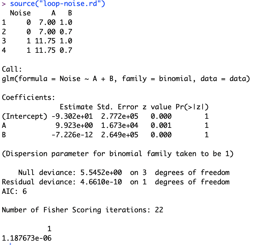
The results looked like:
This tells you:
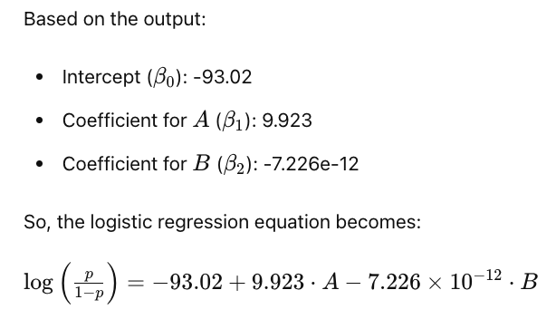
(To compute the probability take the exponential, divide that by 1 + exp(...) In the script below I set A = 8, B = 0.85, and probability came out at essentially 0)
Here is the Script:
# Load necessary library
library(ggplot2)

# Create a dataframe with the new data
data <- data.frame(
  Noise = c(0, 0, 1, 1),
  A = c(7, 7, 11.75, 11.75),
  B = c(1, 0.7, 1, 0.7)
)

# Print the data to verify
print(data)

# Fit logistic regression model
log_model <- glm(Noise ~ A + B, family = binomial, data = data)

# Summary of the model
summary(log_model)

# Print summary of the model
print(summary(log_model))

# Create a scatter plot of Noise vs. A and B
ggplot(data, aes(x = A, y = Noise)) +
  geom_point(aes(color = as.factor(B))) +
  labs(x = "A", y = "Noise", color = "B") +
  theme_minimal()

# Predict probabilities using the logistic regression model
predicted_probs <- predict(log_model, type = "response")

# Create a new data frame with A and B values and predicted probabilities
predicted_data <- data.frame(A = data$A, B = data$B, Predicted_Prob = predicted_probs)

# Plot the predicted probabilities against the A and B variables
ggplot(predicted_data, aes(x = A, y = Predicted_Prob, color = as.factor(B))) +
  geom_point() +
  labs(x = "A", y = "Predicted Probability", color = "B") +
  theme_minimal()

# Predict probability for specific values of A and B
predicted_prob_new <- predict(log_model, newdata = data.frame(A = 8, B = 0.85), type = "response")

# Print the predicted probability
print(predicted_prob_new)
Note: to use R, create the name.rd file, then In Finder (Mac), Navigate to the folder, Open terminal and type pwd In R type: setwd("/path/to/folder") Then type: source("name.rd")